library(rpart)
library(e1071)
library(dplyr)
library(ISLR)

# divide the data into training and testing sets
set.seed(2022)
carseats_index <- sample(x=1:nrow(Carseats), size=0.9*nrow(Carseats), replace=FALSE)
carseats_tr <- Carseats[carseats_index,]
carseats_te <- Carseats[-carseats_index,]

# define a linear regression
carseats_lm <- lm(Sales~., data=carseats_tr)

# define a regression tree (you can also use `adabag::autoprune()`here
carseats_rt <- rpart(Sales~., data=carseats_tr)

# define a support-vector machine
carseats_svm <- svm(Sales ~ ., data=carseats_tr)Variable Importance
Data & models
This exercise shows an example of model-agnostic variable importance for a regression problem. The dataset that we will be working with is Carseats from the ISLR library which has already been used during some of the exercises such as Ex_ML_Tree and Ex_ML_SVM. It is highly recommended that you try to implement some parts of the exercise yourself before checking the answers.
Load the data from ISLR package, then assign 90% of the data for training and the remainder for testing. Please keep in mind that we make a training split running the feature importance (instead of using the entire dataset) as we “may” want to re-train the model with only a fewer features rather than biasing our decision by also including the testing data.
Create three models including a linear regression, a regression tree and a support-vector machine.
Answer
Python
library(reticulate)
use_condaenv("MLBA")
import pandas as pd
import numpy as np
from sklearn.model_selection import train_test_split
from sklearn.linear_model import LinearRegression
from sklearn.tree import DecisionTreeRegressor
from sklearn.svm import SVR
from sklearn.metrics import mean_squared_error
from sklearn.datasets import fetch_openml
# Use the training and test sets created in R (no easy way to get the `Carseats` data in python)
# Convert the categorical columns to one-hot encoded ones
carseats_train, carseats_test = pd.get_dummies(r.carseats_tr.copy()), pd.get_dummies(r.carseats_tr.copy())
# Define a linear regression
carseats_lr = LinearRegression()
carseats_lr.fit(carseats_train.drop(columns=['Sales']), carseats_train['Sales']);
# Define a decision tree regressor
carseats_dtr = DecisionTreeRegressor()
carseats_dtr.fit(carseats_train.drop(columns=['Sales']), carseats_train['Sales']);
# Define a support-vector machine
carseats_svr = SVR()
carseats_svr.fit(carseats_train.drop(columns=['Sales']), carseats_train['Sales']);Variable Importance using DALEX
Feature importance can be manually computed by permuting one column and computing the drop in the value of the loss function (e.g. RMSE for regression and Accuracy for classification). This permutation can be repeated n-times to calculate a mean drop in loss value across various runs. This form of variable importance is often referred to as “permutation feature importance”.
Fortunately, in R there are some nice packages that can help you with that. Three common libraries (among many) for model-agnostic feature importance in R are iml, DALEX and vip . If you would like to learn about the model-specific and model-agnostic feature importance and the various packages in R, you can refer to the chapter 16 of the book “Hands-on Machine Learning with R”. For the purpose of this part of the exercise, we will be using the DALEX library. Please note that the exercise has been largely inspired by the same chapter 16 of the book. You can also check out other variations such as iml and vip implementations.
Creating an explain object
DALEX has an explain object which allows you to do various kind of explanatory analysis. Try reading about the required inputs for it by referring to its documentations (?DALEX::explain()) and also referring to the book mentioned at the beginning of this exercise (“Hands-on Machine Learning with R”). Create one explain object per model for the training data and set the inputs that you need which are model, data (data frame of features) and y (vector of observed outcomes). Also, you can give a caption to your model through the label argument.
library(dplyr)
library(DALEX)

x_train <- select(carseats_tr, -Sales)
y_train <- pull(carseats_tr, Sales)

explainer_lm <- DALEX::explain(model = carseats_lm,
                                 data = x_train,
                                 y = y_train,
                                 label = "Linear Regression")

explainer_rt <- DALEX::explain(model = carseats_rt,
                               data = x_train,
                               y = y_train,
                               label = "Regression Tree")

explainer_svm <- DALEX::explain(model = carseats_svm,
                                data = x_train,
                                y = y_train,
                                label = "Support Vector Machine")
Preparation of a new explainer is initiated
-> model label : Linear Regression
-> data : 360 rows 10 cols
-> target variable : 360 values
-> predict function : yhat.lm will be used ( default )
-> predicted values : No value for predict function target column. ( default )
-> model_info : package stats , ver. 4.4.1 , task regression ( default )
-> predicted values : numerical, min = -0.6248701 , mean = 7.492444 , max = 15.8129
-> residual function : difference between y and yhat ( default )
-> residuals : numerical, min = -2.846017 , mean = -1.865625e-15 , max = 3.3867
A new explainer has been created!
Preparation of a new explainer is initiated
-> model label : Regression Tree
-> data : 360 rows 10 cols
-> target variable : 360 values
-> predict function : yhat.rpart will be used ( default )
-> predicted values : No value for predict function target column. ( default )
-> model_info : package rpart , ver. 4.1.23 , task regression ( default )
-> predicted values : numerical, min = 3.70875 , mean = 7.492444 , max = 12.3904
-> residual function : difference between y and yhat ( default )
-> residuals : numerical, min = -4.03697 , mean = 4.151531e-16 , max = 4.68303
A new explainer has been created!
Preparation of a new explainer is initiated
-> model label : Support Vector Machine
-> data : 360 rows 10 cols
-> target variable : 360 values
-> predict function : yhat.svm will be used ( default )
-> predicted values : No value for predict function target column. ( default )
-> model_info : package e1071 , ver. 1.7.16 , task regression ( default )
-> predicted values : numerical, min = 2.267277 , mean = 7.498075 , max = 15.21856
-> residual function : difference between y and yhat ( default )
-> residuals : numerical, min = -2.780185 , mean = -0.005630512 , max = 2.458701
A new explainer has been created! To calculate the feature importances using Python, we’ll be using the permutation_importance function from the sklearn library.
from sklearn.inspection import permutation_importance
from sklearn.preprocessing import StandardScaler

# Scale the features (relevant to SVM)
scaler = StandardScaler()
carseats_train_scaled = carseats_train.copy()
carseats_test_scaled = carseats_test.copy()

# Calculate feature importances for each model
importance_lr = permutation_importance(carseats_lr, carseats_train.drop(columns=['Sales']), carseats_train['Sales'], n_repeats=10, random_state=2022)
importance_dtr = permutation_importance(carseats_dtr, carseats_train.drop(columns=['Sales']), carseats_train['Sales'], n_repeats=10, random_state=2022)
importance_svr = permutation_importance(carseats_svr, carseats_train.drop(columns=['Sales']), carseats_train['Sales'], n_repeats=10, random_state=2022)
# Train the SVM model on scaled data
carseats_svr_scaled = SVR(kernel='linear')
carseats_svr_scaled.fit(carseats_train_scaled.drop(columns=['Sales']), carseats_train_scaled['Sales']);
importance_svr_scaled = permutation_importance(carseats_svr_scaled, carseats_train_scaled.drop(columns=['Sales']), carseats_train_scaled['Sales'], n_repeats=10, random_state=2022)

# Print the feature importances
importance_df = pd.DataFrame(data={
    'Feature': carseats_train.drop(columns=['Sales']).columns,
    'Linear Regression': importance_lr.importances_mean,
    'Decision Tree': importance_dtr.importances_mean,
    'Support Vector Machine (unscaled)': importance_svr.importances_mean,
    'Support Vector Machine (scaled)': importance_svr_scaled.importances_mean
})

print(importance_df)
Feature ... Support Vector Machine (scaled)
0 CompPrice ... 0.437965
1 Income ... 0.051003
2 Advertising ... 0.156785
3 Population ... 0.000136
4 Price ... 1.146152
5 Age ... 0.152260
6 Education ... 0.001026
7 ShelveLoc_Bad ... 0.232378
8 ShelveLoc_Good ... 0.257843
9 ShelveLoc_Medium ... 0.004519
10 Urban_No ... 0.000531
11 Urban_Yes ... 0.000531
12 US_No ... 0.000160
13 US_Yes ... 0.000160
[14 rows x 5 columns]You can observe the value of scaling for SVM. The results seems to agree that Price is the most important feature.
Plotting the feature importance
Now that you have created the DALEX::explain objects, we will use another function called model_parts which takes care of the feature permutation. Try reading about the function DALEX::model_parts() . The main arguments that you need to provide to the explain function are:
An
explainerobject (what you created above).Bwhich is the number of permutations (i.e. how many times you want to randomly shuffle each column).The
typeof scores you would like it to return (raw score vs differences vs ratios) which in this case we set toratioand you can read more the differences in the documentation.Nargument which you can set toN=NULLwhich essentially asks how many samples you would like to use for calculating the variable importance, where setting it toNULLmeans that we use the entire training set.There is also a
loss_functionwhich by default isRMSEfor regression (our case) and1-AUCfor classification, by there are a few more which you can find out about by referring to the documentations (e.g. through?DALEX::loss_root_mean_square).
After assigning model_parts to a variable, try plotting each model to see the most important variables. What do you see? Are there important features that are in common?
calculate_importance <- function(your_model_explainer, n_permutations = 10) {
  imp <- model_parts(explainer = your_model_explainer,
                     B = n_permutations,
                     type = "ratio",
                     N = NULL)
  return(imp)
}

importance_lm  <- calculate_importance(explainer_lm)
importance_rt  <- calculate_importance(explainer_rt)
importance_svm <- calculate_importance(explainer_svm)

library(ggplot2)
plot(importance_lm, importance_rt, importance_svm) +
  ggtitle("Mean variable-importance ratio over 10 permutations", "")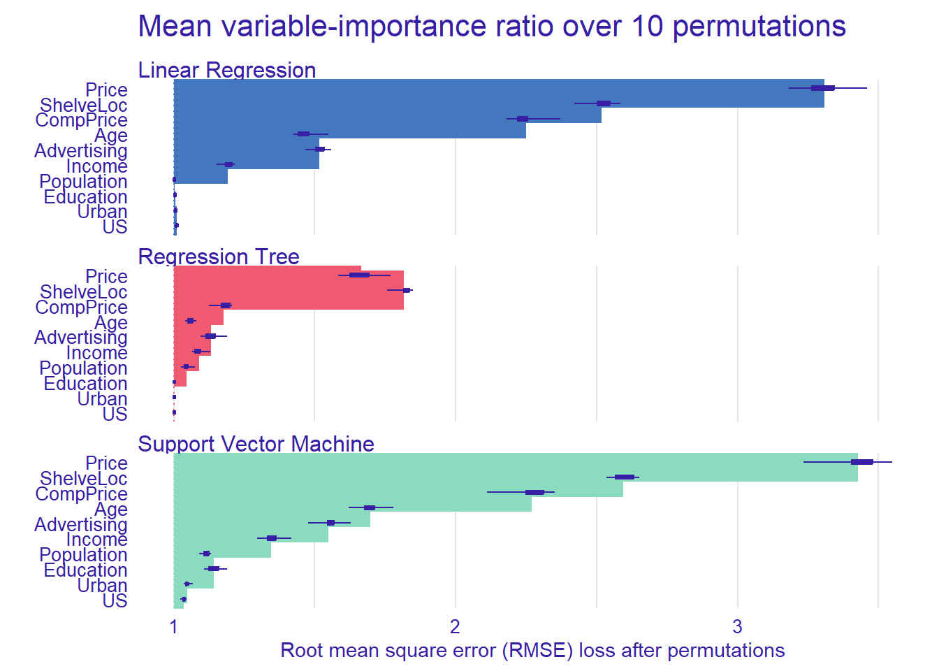
Partial Dependence Plots (PDP)
Partial dependence plots (PDPs) show the marginal effect of one or two features on the predicted outcome of a machine learning model. They can be used to visualize and interpret the influence of selected features on the model’s predictions. We’ll continue using the same Carseats data. We first create PDPs for the Price and Advertising features using the the SVM model carseats_svm created earlier:
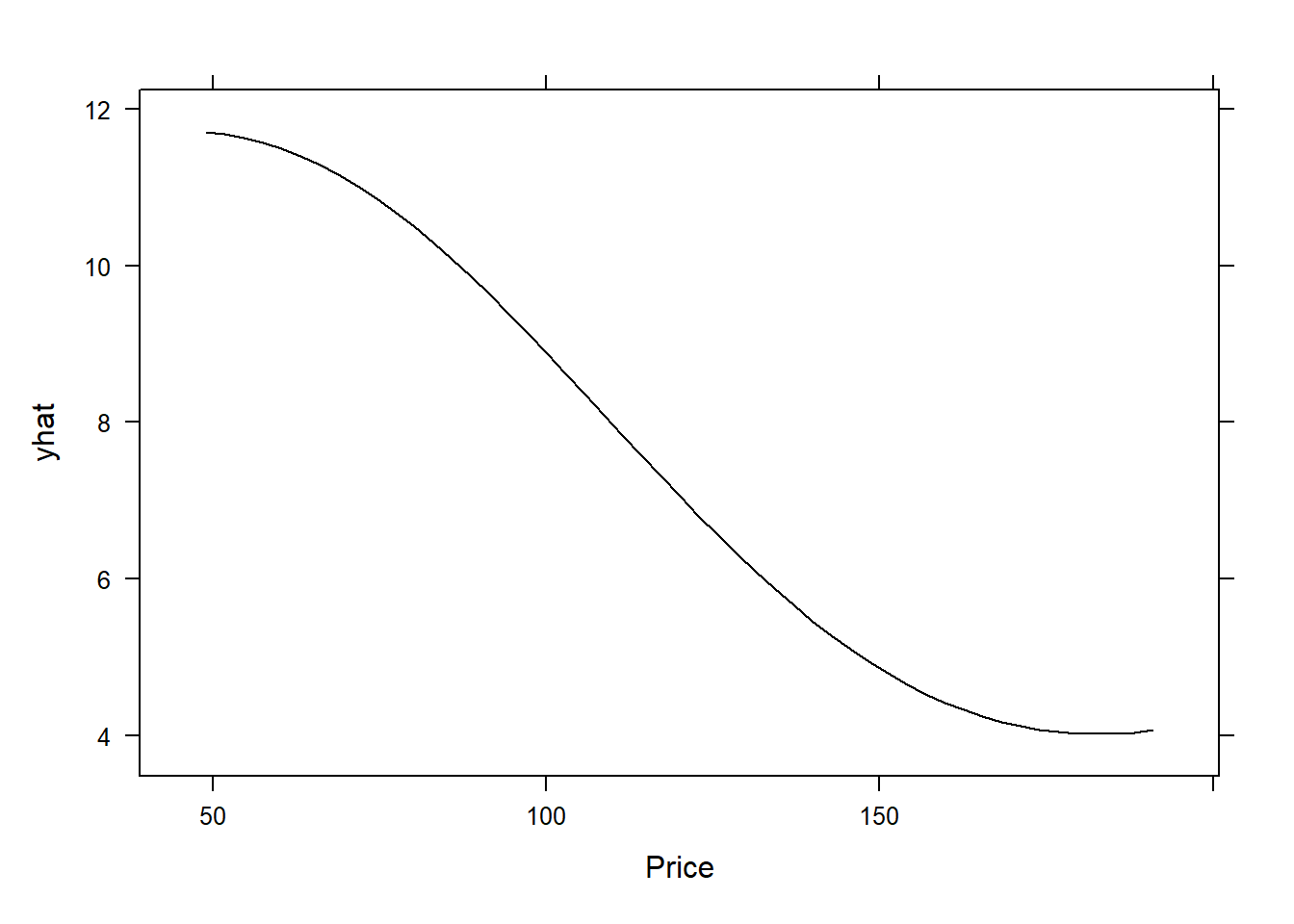
pdp::partial(carseats_svm, pred.var = "Advertising", plot = TRUE)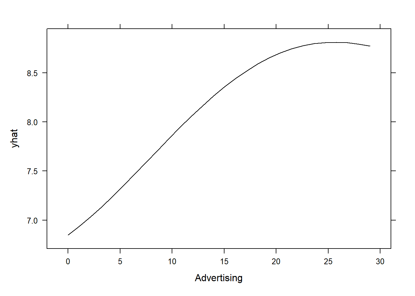
What we see in the first plot is that for this particular model, the higher the price, the number of carseats sold (units) which makes sense. With regards to the advertising, we see that the higher the local advertising budget for the company (see ?Carseats for more details), the higher the sales number of units for a car, however, there’s a plateau after which you cannot sell more units. This means that after a certain point, increasing the advertising budget may no longer bring any benefit in terms of the units sold. It’s important to note that in PDP, we study the decision by the model and not the data, however, we can always visualize our results to see if they follow a similar trend or not:
# plot(Carseats$Advertising, Carseats$Sales, xlab = "Advertising Budget", ylab = "Sales Units")
ggplot(data = carseats_tr, aes(x = Advertising, y = Sales)) +
  geom_point() +
  labs(x = "Advertising Budget", y = "Sales Unit") +
  ggtitle("Relationship between Sales and Advertising Budget")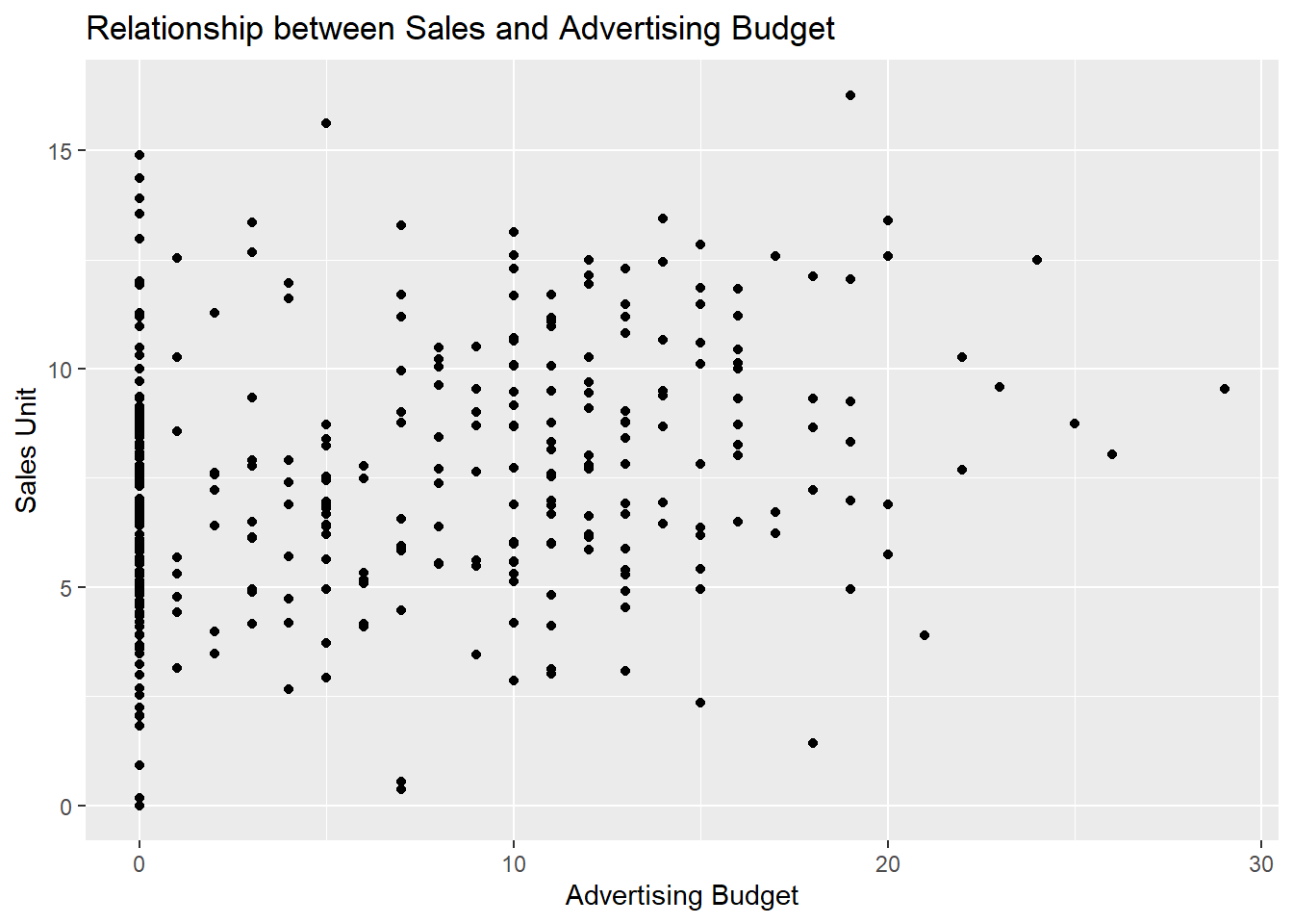
We can see that the trend is not very clear but may be headed in the same direction.
For categorical features, such as ShelveLoc, we can make a similar kind of PDP:
pdp::partial(carseats_svm, pred.var = "ShelveLoc", plot = TRUE, plot.engine = "ggplot")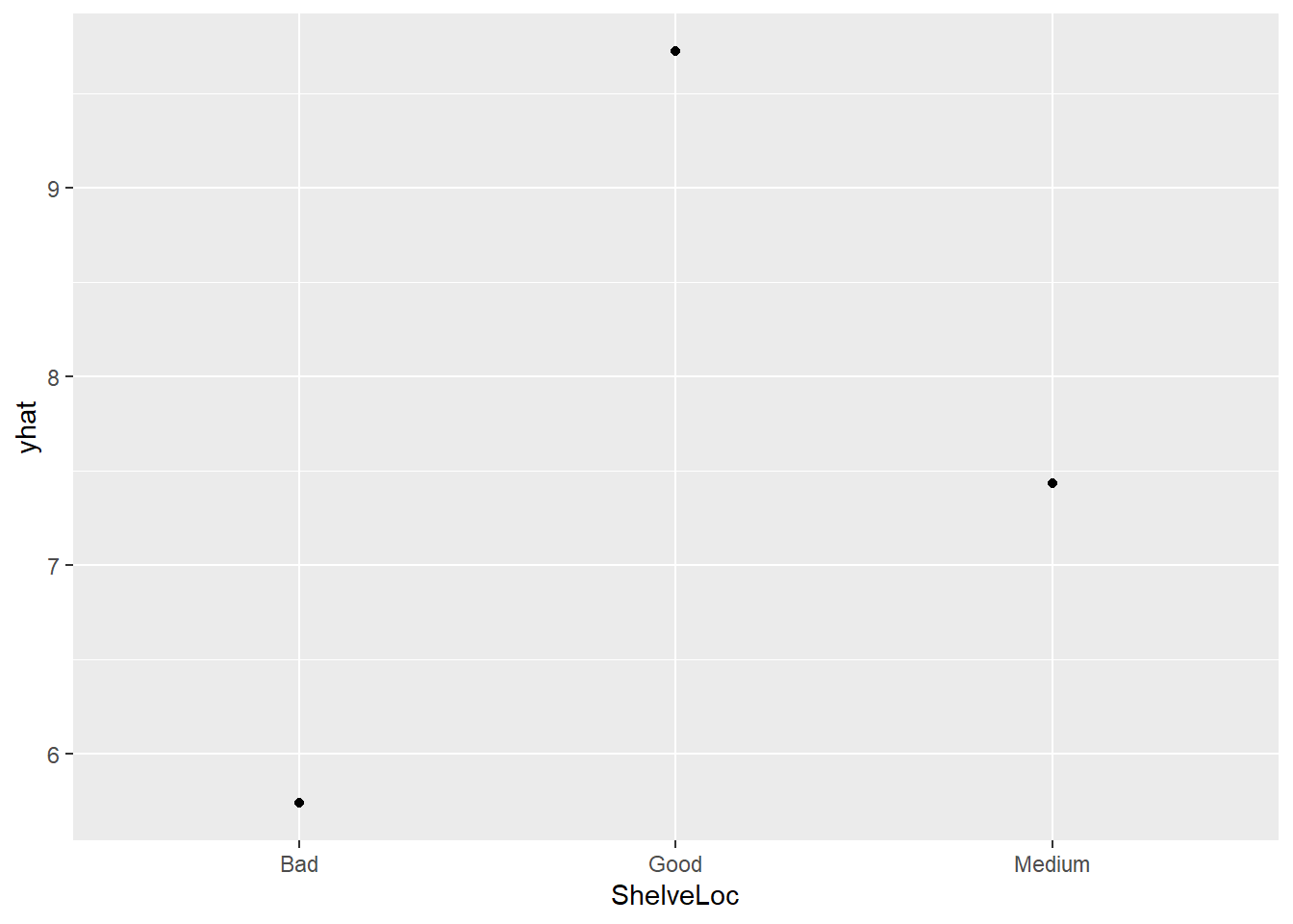
From this plot, we can see that the better the quality of shelving location, the high the number of units sold (which again makes sense).
PDPs can have some limitations, which you, as users, should be aware of. These limitations do partially apply to other techniques presented during lab:
Assuming feature independence: PDPs assume that the features being plotted are independent of each other. This can lead to misleading results when there is a strong correlation or interaction between features, as the partial dependence function will not capture their combined effect accurately.
Inaccurate representation of complex interactions: PDPs cannot represent high-order interactions or nonlinear relationships between features.
Unreliable in the presence of outliers: PDPs can be sensitive to outliers and extreme values in the dataset, which may result in distorted representations of the feature’s impact on the model’s predictions. Proper preprocessing and outlier detection techniques should be employed to avoid this issue.
Using the average values: PDPs uses the mean expected value for the final prediction of the target feature. This should be fine in most applications, but it may be inappropriate in some applications.
Computational burden: Generating PDPs can be computationally expensive, especially for high-dimensional datasets or complex models. It is important to weigh the benefits of this technique against the computational resources available.
Keep in mind these limitations when interpreting PDPs (and other techniques) and consider these limitations when drawing conclusions from them.
We can now create a two-way PDP to explore the interaction between Price and Advertising:
pdp::partial(carseats_svm, pred.var = c("Price", "Advertising"), plot = TRUE)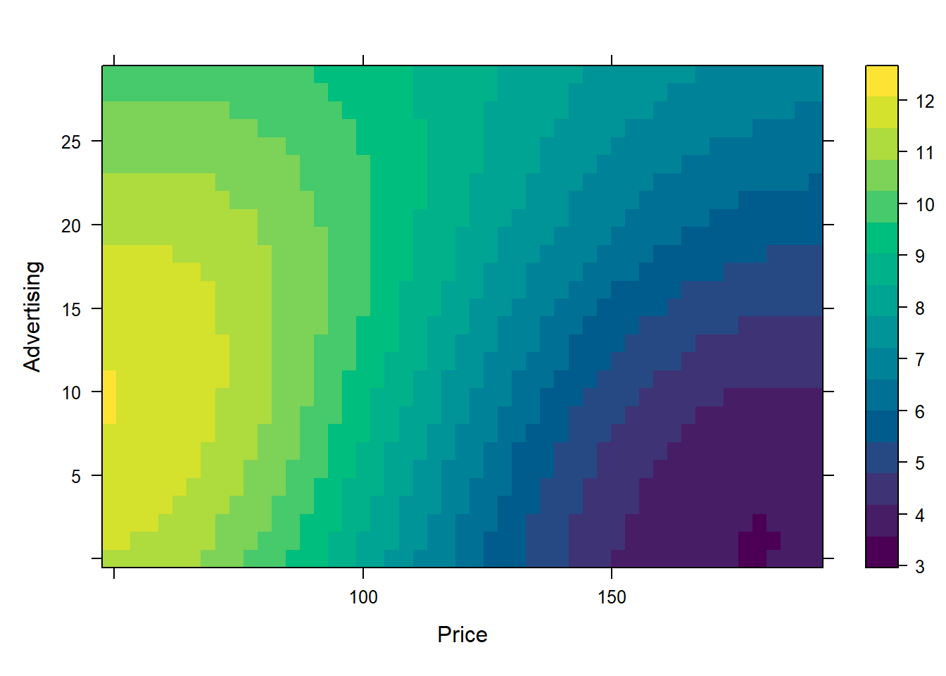
A combination of moderate advertising (around 2-18) and low prices (from around 0-40) seems to produce the highest sales units by the SVM model.
You may note how no python implementation of PDP has been shown since sklearn.inspection.plot_partial_dependence, which was suitable for this task, has recently changed, and the new alternative does not always work well for categorical variables. However, if you are interested, feel free to look up existing alternatives.
LIME (Local Interpretable Model-agnostic Explanations)
LIME helps explain individual predictions of machine learning models by fitting a local, interpretable model around a specific data point. This allows for more transparency and understanding of the model’s behavior for individual instances.
SVM
lime package does not support the SVM model from the e1071 package out of the box.You can see the list of supported models via ?model_type. There are solutions to this:
- Re-train your model with the
caretlibrary which we then work directly with this library (also may be good practice to build your models withcaret).
# Load the lime library
library(lime)

# Create a caret model using a support vector machine
svm_caret_model <- caret::train(Sales ~ ., data = carseats_tr, method = "svmLinear2", trControl = trainControl(method = "none"))

# Predict on a test instance
test_instance <- carseats_te[1:4, -1]

# Create a lime explainer object for the SVM model
lime_svm_explainer <- lime::lime(carseats_tr[, -1],
                                 svm_caret_model)

# Explain a prediction using lime
lime_svm_explanation <- explain(test_instance, lime_svm_explainer, n_features = 10)
plot_features(lime_svm_explanation)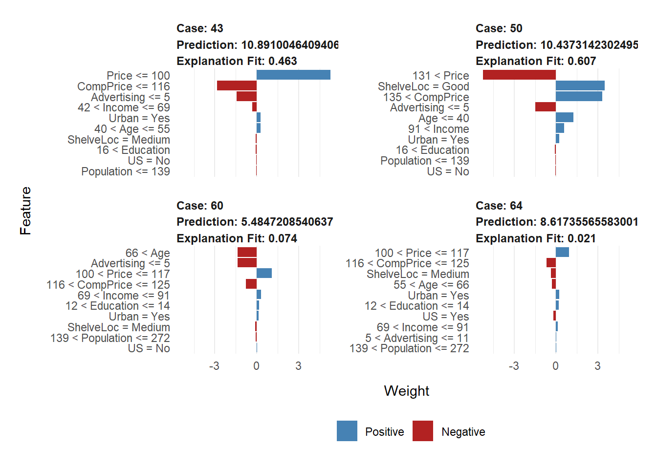
- Create custom
predict_modelandmodel_typemethods for the SVM model.
# Custom predict_model function for SVM
predict_model.svm <- function(x, newdata, type, ...) {
  if (type == "raw") {
    res <- predict(x, newdata = newdata, ...)
    return(data.frame(Response = res, stringsAsFactors = FALSE))
  } else if (type == "prob") {
    res <- predict(x, newdata = newdata, ...)
    prob <- kernlab::kernel(x, newdata, j = -1)
    return(as.data.frame(prob, check.names = FALSE))
  }
}

# Custom model_type function for SVM
model_type.svm <- function(x, ...) {
  if (x$type == "C-classification") {
    return("classification")
  } else {
    return("regression")
  }
}

# Create a LIME explainer for the SVM model
lime_svm_explainer <- lime(x_train, carseats_svm)

# Choose a specific instance from the test set to explain
test_instance <- carseats_te[1:4,-1]

# Generate explanations for the chosen instance
lime_svm_explanation <- explain(test_instance, lime_svm_explainer, n_features = 10)

# Visualize the explanation
plot_features(lime_svm_explanation)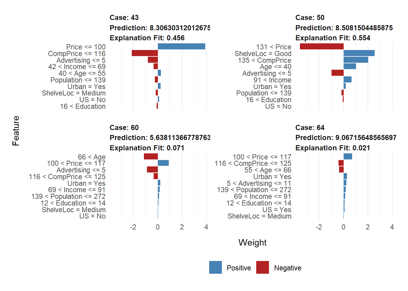
You can see the prediction plot for 4 test observations. We can see several bar charts. On the y-axis, you see the features (and their intervals), while the x-axis shows the relative strength of each feature at a given value or interval. The positive value (blue color) shows that the feature support or increases the value of the prediction, while the negative value (red color) has a negative effect or decreases the prediction value. Please note that the interpretation for each observation can be different (this explanation has been taken from this blog, which you can visit for further details).
We give the interpretation of the first test observation as an example. The first subplot shows that a price of less than 100 results in purchasing a higher quantity than expected. Additionally, people between the ages of 40 and 55 were most likely to buy the seat, which are people who are not too young nor too old. However, in a typical scenario, we would generally expect younger people to buy car seats, but that’s probably because of the high ages in our dataset (1st. quantile of age is around 40). If the price by the competitor (CompPrice) is also low, it’ll impact the sales units badly. Once again, please note that this is specific to the first observation (i.e., the first subplot).
The next element is Explanation Fit. These values indicate how well LIME explains the model, similar to an R-Squared in linear regression. Here we see the explanation Fit only has values around 0.50-0.7 (50%-70%), which can be interpreted that LIME can only explain a little about our model (in some cases, like the 3rd sub-plot, this value is extremely low). You may choose not to trust the LIME output since it only has a low Explanation Fit.
We’ll be using provide a small demonstration on how this can be achieved in python. Please note the same logic for the interpretation (and explanation) of the R version applies here, therefore, the code is shorter and there’s no further comment provided for its output.
We use lime package in python (already installed in the lab setup). Then we can run our model in the same way as R:
from sklearn import svm
from sklearn.pipeline import make_pipeline
from lime import lime_tabular
import matplotlib.pyplot as plt

# Assuming carseats_tr and carseats_te are already defined as pandas DataFrames
X_train = carseats_train.drop(columns='Sales')
y_train = carseats_train['Sales']
X_test = carseats_test.drop(columns='Sales')

# Create a support vector machine model
svm_caret_model = svm.LinearSVR(random_state=2022)

# Train the model
svm_caret_model.fit(X_train, y_train);

# Predict on a test instance
test_instance = X_test.iloc[0:4]

# Create a lime explainer object for the SVM model
lime_svm_explainer = lime_tabular.LimeTabularExplainer(X_train.values,
                                                       feature_names=X_train.columns,
                                                       class_names=['Sales'],
                                                       mode='regression')

# Explain a prediction using lime
lime_svm_explanation = lime_svm_explainer.explain_instance(test_instance.values[0], svm_caret_model.predict, num_features=10)

# Plot the features
# plt.clf()
lime_svm_explanation.as_pyplot_figure()
plt.show()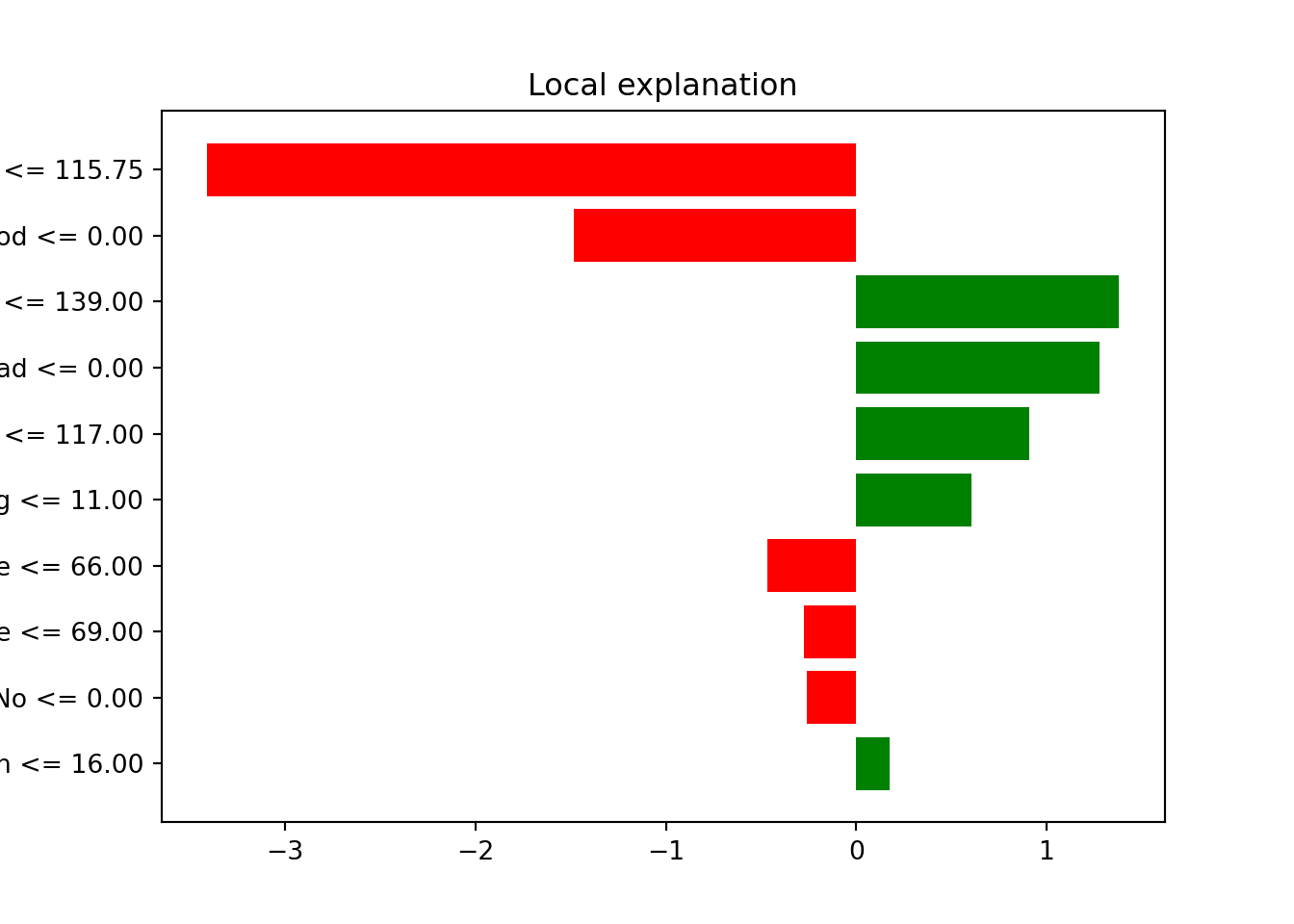
Bonus: XGBoost
To give you an example for a classification problem, we can also train an XGBoost using the xgboost library:
library(xgboost)

# Load and prepare the data
carseats_df <- Carseats
carseats_df$High <- ifelse(carseats_df$Sales <= 8, "yes", "no")
carseats_df$High <- as.factor(carseats_df$High)
carseats_df$ShelveLoc <- as.factor(carseats_df$ShelveLoc)
carseats_df$Urban <- as.factor(carseats_df$Urban)
carseats_df$US <- as.factor(carseats_df$US)

# Prepare the data for xgboost (as shown in the boosting excercises)
xgb_data <- model.matrix(High ~ ., data = carseats_df)[,-1]
xgb_label <- as.numeric(carseats_df$High) - 1
xgb_dmatrix <- xgb.DMatrix(data = xgb_data, label = xgb_label)

# Train a gradient boosting model
set.seed(42)
carseats_xgb <- xgboost(data = xgb_dmatrix, nrounds = 100, objective = "binary:logistic", eval_metric = "logloss")
[1] train-logloss:0.441670
[2] train-logloss:0.301386
[3] train-logloss:0.212602
[4] train-logloss:0.153032
[5] train-logloss:0.111713
[6] train-logloss:0.082449
[7] train-logloss:0.061431
[8] train-logloss:0.046187
[9] train-logloss:0.035048
[10] train-logloss:0.026860
[11] train-logloss:0.020809
[12] train-logloss:0.016314
[13] train-logloss:0.012954
[14] train-logloss:0.010426
[15] train-logloss:0.008509
[16] train-logloss:0.007042
[17] train-logloss:0.005908
[18] train-logloss:0.005021
[19] train-logloss:0.005013
[20] train-logloss:0.005008
[21] train-logloss:0.005005
[22] train-logloss:0.005003
[23] train-logloss:0.005002
[24] train-logloss:0.005001
[25] train-logloss:0.005000
[26] train-logloss:0.005000
[27] train-logloss:0.005000
[28] train-logloss:0.004999
[29] train-logloss:0.004999
[30] train-logloss:0.004999
[31] train-logloss:0.004999
[32] train-logloss:0.004999
[33] train-logloss:0.004999
[34] train-logloss:0.004999
[35] train-logloss:0.004999
[36] train-logloss:0.004999
[37] train-logloss:0.004999
[38] train-logloss:0.004999
[39] train-logloss:0.004999
[40] train-logloss:0.004999
[41] train-logloss:0.004999
[42] train-logloss:0.004999
[43] train-logloss:0.004999
[44] train-logloss:0.004999
[45] train-logloss:0.004999
[46] train-logloss:0.004999
[47] train-logloss:0.004999
[48] train-logloss:0.004999
[49] train-logloss:0.004999
[50] train-logloss:0.004999
[51] train-logloss:0.004999
[52] train-logloss:0.004999
[53] train-logloss:0.004999
[54] train-logloss:0.004999
[55] train-logloss:0.004999
[56] train-logloss:0.004999
[57] train-logloss:0.004999
[58] train-logloss:0.004999
[59] train-logloss:0.004999
[60] train-logloss:0.004999
[61] train-logloss:0.004999
[62] train-logloss:0.004999
[63] train-logloss:0.004999
[64] train-logloss:0.004999
[65] train-logloss:0.004999
[66] train-logloss:0.004999
[67] train-logloss:0.004999
[68] train-logloss:0.004999
[69] train-logloss:0.004999
[70] train-logloss:0.004999
[71] train-logloss:0.004999
[72] train-logloss:0.004999
[73] train-logloss:0.004999
[74] train-logloss:0.004999
[75] train-logloss:0.004999
[76] train-logloss:0.004999
[77] train-logloss:0.004999
[78] train-logloss:0.004999
[79] train-logloss:0.004999
[80] train-logloss:0.004999
[81] train-logloss:0.004999
[82] train-logloss:0.004999
[83] train-logloss:0.004999
[84] train-logloss:0.004999
[85] train-logloss:0.004999
[86] train-logloss:0.004999
[87] train-logloss:0.004999
[88] train-logloss:0.004999
[89] train-logloss:0.004999
[90] train-logloss:0.004999
[91] train-logloss:0.004999
[92] train-logloss:0.004999
[93] train-logloss:0.004999
[94] train-logloss:0.004999
[95] train-logloss:0.004999
[96] train-logloss:0.004999
[97] train-logloss:0.004999
[98] train-logloss:0.004999
[99] train-logloss:0.004999
[100] train-logloss:0.004999 Identify instances with predicted probabilities close to 1, 0, and 0.5:
[1] 4
[1] 1
[1] 1
Generate LIME explanations for the selected instances:
# before making the prediction, we need to also one-hot encode the categorical variables
to_explain <- data.frame(model.matrix(~.,data = carseats_df[c(120, 4, 60), -ncol(carseats_df)])[,-1])

# we can finally run LIME on our results
carseats_lime_xgb <- lime(data.frame(xgb_data), carseats_xgb, bin_continuous = TRUE, quantile_bins = FALSE)
carseats_expl_xgb <- lime::explain(to_explain, carseats_lime_xgb, n_labels = 1, n_features = 10)
Visualize the LIME explanations
plot_features(carseats_expl_xgb, ncol = 2)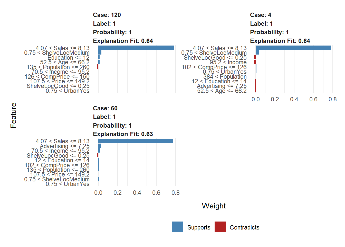
What can you observe from these subplots?
Your turn
After having done this for the training set, make a selection of the most important variables and run the model again. Would you go for this simpler model that has less features or the more complicated one? (hint: you can compute some scores to see whether dropping features would justify the performance drop).
As a final remark, the same kind of analysis can also be done for classification and different loss functions.
