---
title: "Models: Linear and logistic regressions"
output-file: Ex_ML_LinLogReg.html
---
```{r global_options, include = FALSE}
knitr::opts_chunk$set(fig.align="center", results = 'hold', fig.show = 'show', warning = FALSE, message = FALSE)
```
# Linear regression: real estate application
The dataset we'll be using for the first part of the exercise is real estate transaction prices in Taiwan, which can be accessed from this link [this link](https://archive.ics.uci.edu/ml/datasets/Real+estate+valuation+data+set). This dataset was modified for this exercise. The modified file `real_estate_data.csv` is in the exercise folder under `/data/`.
The aim is to predict the house prices from available features: *No*, *Month*, *Year*, *TransDate*, *HouseAge*, *Dist*, *NumStores*, *Lat*, *Long*, *Price*. *No* is the transaction number and will not be used.
## EDA
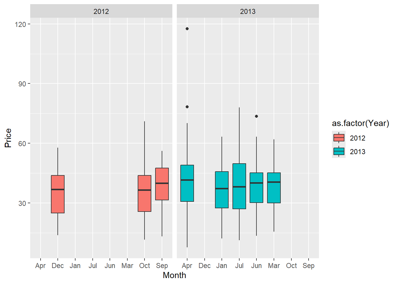
First, an EDA of the data is needed. After exploring the structure, the *Price* is shown with the year and month.
```{r}
real_estate_data <- read.csv(here::here("labs/data/real_estate_data.csv"))

## adapt the path to the data
# if you encountered any error with the encoding of the data (`Error in gregexpr...`), just re-run the code again
str(real_estate_data)
library(summarytools)
dfSummary(real_estate_data)

library(dplyr)
library(ggplot2)
real_estate_data %>% ggplot(aes(x=Month, y=Price, fill=as.factor(Year))) +
  geom_boxplot()+ facet_wrap(~as.factor(Year))
```
The results show how important it is to make an EDA! It appears that the data does not contain transactions for all the months of 2012 and 2013, but just some months by the end of 2012 and the first half of 2013. This shows that it is pointless to use month and year here. This is why we prefer *TransDate*, a value indicating the transaction time on a linear scale (e.g., 2013.250 is March 2013).
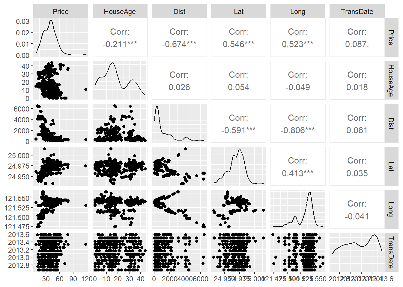
Now we focus on the link between *Price* and the other features.
```{r}
library(GGally)
real_estate_data %>%
  select(Price, HouseAge, Dist, Lat, Long, TransDate) %>%
  ggpairs()
```
No clear link appears. The linear regression will help to discover if a combination of the features can predict the price.
## Modelling
First, we split the data into training/test set (75/25).
```{r}
set.seed(234)
index <- sample(x=c(1,2), size=nrow(real_estate_data), replace=TRUE, prob=c(0.75,0.25)) # 1==training set, 2==test set
dat_tr_restate <- real_estate_data[index==1,]
dat_te_restate <- real_estate_data[index==2,]
```
Then, we fit the linear regression to the training set.
::: panel-tabset
### R
```{r}
mod_lm <- lm(Price~TransDate+
               HouseAge+
               Dist+
               NumStores+
               Lat+
               Long, data=dat_tr_restate)
summary(mod_lm)
```
### Python
```{r}
#| label: load-conda
# In R, we load the conda environment as usual
library(reticulate)
reticulate::use_condaenv("MLBA", required = TRUE)
gc(full = TRUE)
```
In python, we then use the `statsmodels` library to fit a linear regression model to the training data and perform feature elimination. We use the `.fit()` method to fit the model with the formula for the variable names. Note that python's `summary()` function is unique to the `statsmodels` libraries and produces similar information to its R counterpart.
```{python import-mkl}
import os
os.environ["OMP_NUM_THREADS"] = "1"
os.environ["MKL_NUM_THREADS"] = "1"

import mkl
# %env OMP_NUM_THREADS=1
# set the number of threads. Here we set it to 1 to avoid parallelization when rendering quarto, but you can set it to higher values.
mkl.set_num_threads(1)
```
```{python stats-import}
# Import necessary library
import statsmodels.formula.api as smf

# Fit a linear regression model to the training data & print the summary
mod_lm_py = smf.ols(formula='Price ~ TransDate + HouseAge + Dist + NumStores + Lat + Long', data=r.dat_tr_restate).fit()
print(mod_lm_py.summary())
```
It's not a suprise that the results are same as the ones obtained in R.
:::
## Variable selection & interpretation
The stepwise variable selection can be performed using the function **step**. By default, it is a backward selection; see `?step` for details (parameter **direction** is **backward** when **scope** is empty).
::: panel-tabset
### R
```{r}
step(mod_lm) # see the result
mod_lm_sel <- step(mod_lm) # store the final model into mod_lm_sel
summary(mod_lm_sel)
```
### Python
As python does not have an exact equivalent of `stats::step()` function, which performs both forward and backward selection based on AIC, we have to implement it manually. We start with the full model and iteratively remove the feature with the highest p-value and add the feature with the lowest AIC until we can no longer improve the AIC. The final model is stored in `mod_lm_sel`. For an extensive explanation of what this while loop is doing and how the backward+forward is computed, check the code below:
<details>
<summary>Explaining feature elimination in python (while loop) </summary>
We start by setting `mod_lm_sel_py` to the full model `mod_lm_py`. Then, we enter a while loop that continues until we break out of it. In each iteration of the loop, we store the current model in prev_model for later comparison. We start by dropping the feature with the highest p-value from the current model using `idxmax()`, which returns the label of the maximum value in the pvalues attribute of the `mod_lm_sel_py` object. We exclude the intercept term from the list of labels by specifying `labels=['Intercept']`. We then create a new model using `smf.ols()` with the feature removed and fit it to the training data using `fit()`. We store this new model in `mod_lm_sel_py`.
Next, we check whether the AIC of the new model is larger than the previous model's. If it is, we break out of the while loop and use the previous model (prev_model) as the final model. If not, we continue to the next step of the loop. Here, we look for the feature with the lowest AIC among the remaining features using `idxmin()` on the pvalues attribute, again excluding the intercept term. We create a new model by adding this feature to the current model using `smf.ols()`, fit it to the training data using `fit()`, and store it in `mod_lm_sel_new`.
We then check whether the AIC of the new model is larger than that of the current model. If it is, we break out of the while loop and use the current model (`mod_lm_sel_py`) as the final model. If not, we update `mod_lm_sel_py` with the new model and continue to the next iteration of the loop. This way, we iteratively remove the feature with the highest p-value and add the feature with the lowest AIC until we can no longer improve the AIC. The final model is stored in `mod_lm_sel_py`.
</details>
```{python stats-stepwise}
import statsmodels.api as sm
import matplotlib.pyplot as plt

# perform both forward and backward selection using AIC
mod_lm_sel_py = mod_lm_py

while True:
    prev_model = mod_lm_sel_py
    # drop the feature with the highest p-value
    feature_to_drop = mod_lm_sel_py.pvalues.drop(labels=['Intercept']).idxmax()
    mod_lm_sel_py = smf.ols(formula='Price ~ TransDate + HouseAge + Dist + NumStores + Lat + Long - ' + feature_to_drop, data=r.dat_tr_restate).fit()
    # check if AIC has increased, if yes, break the loop and use the previous model
    if mod_lm_sel_py.aic > prev_model.aic:
        mod_lm_sel_py = prev_model
        break

    # add the feature with the lowest AIC
    feature_to_add = mod_lm_sel_py.pvalues.drop(labels=['Intercept']).idxmin()
    mod_lm_sel_py_new = smf.ols(formula='Price ~ TransDate + HouseAge + Dist + NumStores + Lat + Long + ' + feature_to_add, data=r.dat_tr_restate).fit()
    # check if AIC has increased, if yes, break the loop and use the previous model
    if mod_lm_sel_py_new.aic > mod_lm_sel_py.aic:
        break
    mod_lm_sel_py = mod_lm_sel_py_new

print(mod_lm_sel_py.summary())
```
:::
After identifying the most important features, you can fit a new model using only those features and evaluate its performance using the test set.
The final model does not contain *Long*. In terms of interpretations, for example:
- The price increased on average by 3.7 per year (*TransDate*)
- It diminishes in average by (-2)2.4 per year (*HouseAge*)
- etc.
## Inference
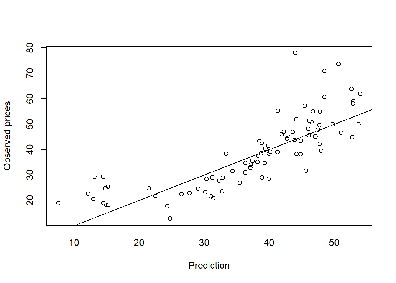
We now predict the prices in the test set. We can make a scatter plot of the predictions versus the observed prices to inspect that. We already know by looking at the $R^2$ in the summary that the prediction quality is not good.
::: panel-tabset
### R
```{r}
mod_lm_pred <- predict(mod_lm_sel, newdata=dat_te_restate)
plot(dat_te_restate$Price ~ mod_lm_pred, xlab="Prediction", ylab="Observed prices")
abline(0,1) # line showing the obs -- pred agreement
```
### Python
```{python}
#| label: predict-output
#| eval: false
mod_lm_sel_pred = mod_lm_sel_py.predict(r.dat_te_restate)
fig, ax = plt.subplots()
ax.scatter(x=mod_lm_sel_pred, y=r.dat_te_restate['Price']);
ax.set_xlabel('Prediction');
ax.set_ylabel('Observed prices');
ax.plot(ax.get_xlim(), ax.get_ylim(), ls="--", c=".3");
plt.show()
```
:::
It appears that the lowest and the highest prices are underestimated. At the center (around 30), the prices are slightly overestimated.
As an exercise, write down the prediction equation of the selected model. Use this equation to explain how instances 1 and 2 (test set) are predicted and calculate the predictions manually. Verify your results using the *predict* function from the previous R code.
<details>
<summary>Answer</summary>
```{r}
#| label: show-model-output
mod_lm_pred[c(1,2)]
```
$$
y = -0.000133 + 3.66\times TransDate -0.243\times HouseAge \\-0.00464\times Dist + 1.027\times NumStores + 237.8\times Lat
$$
</details>
# Logistic regression: visit data
To illustrate a logistic regression, we use the data set **DocVis** extracted (modified for the exercise) the library **AER**. The data set reports a 1977--1978 Australian Health Survey. The aim is to predict the outcome **visits**, a binary variable indicating if the individual had at least one visit to a doctor in the past two weeks, using all the other features. To learn more about these features, look at the data described below.
<details>
<summary>Data Description</summary>
The predictors are as followed:
- gender: M/F
- age: Age in years divided by 100.
- income: Annual income in tens of thousands of dollars.
- illness: Number of illnesses in past 2 weeks.
- reduced: Number of days of reduced activity in past 2 weeks due to illness or injury.
- health: General health questionnaire score using Goldberg's method.
- private: Factor. Does the individual have private health insurance?
- freepoor: Factor. Does the individual have free government health insurance due to low income?
- freerepat: Factor. Does the individual have free government health insurance due to old age, disability or veteran status?
- nchronic: Factor. Is there a chronic condition not limiting activity?
- lchronic: Factor. Is there a chronic condition limiting activity?
</details>
We can now load the dataset.
```{r}
DocVis <- read.csv(here::here("labs/data/DocVis.csv")) ## found in the same data folder
```
To facilitate the use of logistic regression in **R**, it is **strongly recommended** to have a 0/1 outcome rather than a categorical one. This makes much easier the recognition of the positive label (the "1") and the negative one (the "0"). Since we want to predict **visits**, we transform it accordingly.
```{r}
DocVis$visits <- ifelse(DocVis$visits=="Yes",1,0)
```
## Modelling
We can split our data and fit the logistic regression. The function for this is **glm**. This function encompasses a larger class of models (namely, the generalized linear models) which includes the logistic regression, accessible with **family="binomial"**.
```{r}
set.seed(234)
index <- sample(x=c(1,2), size=nrow(DocVis), replace=TRUE, prob=c(0.75,0.25)) # 1==training set, 2==test set
dat_tr_visit <- DocVis[index==1,]
dat_te_visit <- DocVis[index==2,]
```
::: panel-tabset
### R
```{r}
vis_logr <- glm(visits~., data=dat_tr_visit, family="binomial")
summary(vis_logr)
```
### Python
```{python}
# a hack around this technique to not type all the variable names
vis_formula = 'visits ~ ' + ' + '.join(r.dat_tr_visit.columns.difference(['visits']))

# create a logistic regression model
vis_logr_py = sm.formula.logit(formula= vis_formula, data=r.dat_tr_visit).fit()

print(vis_logr_py.summary())
```
::: callout-warning
# Using `.` for formulas in R vs Python
In R, the dot `.` is used as shorthand to indicate that we want to include all other variables in the formula as predictors except for the outcome variable. So, if our outcome variable is y and we want to include all other variables in our data frame as predictors, we can write `y ~ .` in the formula.
In Python, however, the dot `.` is not used in the same way in formulas. Instead, to include all other variables as predictors except for `y`, we would write `y ~ x1 + x2 + ...` where `x1, x2`, etc. represent the names of the predictor variables. Also, `statsmodels` has a similar syntax to R base regressions. In most other typical ML libraries in Python, you must provide the column values instead of using the column names.
:::
Note that the `family="binomial"` argument in R is not needed in Python since `sm.formula.logit()` assumes the logistic regression model is fitted using a binomial distribution by default.
:::
## Variable selection & interpretation
Now, we can apply the variable selection:
::: panel-tabset
### R
```{r}
vis_logr_sel <- step(vis_logr)
summary(vis_logr_sel)
```
### Python
As already seen in the linear regression part, in python, we don't have the same implementation of the step function, hence why we designed the while loop earlier. It is good practice to create a single function with this step while loop to handle all cases (linear, logistic etc); however, we only implement it here for logistic regression. Therefore, to tackle this, we will create a function that does step-wise elimination for us. We define a function called `forward_selected` that performs forward selection on a given dataset to select the best predictors for a response variable based on AIC. The function takes two arguments: `data`, a pandas DataFrame containing the predictors and `response` variable, and response, a string specifying the name of the response variable.
<details>
<summary>For more explanation of the code, click on me</summary>
The function first initializes two sets: `remaining` and `selected`. `remaining` contains the names of all columns in the `data` DataFrame except for the `response` variable, while `selected` is initially empty. The function then initializes `current_aic` and `best_new_aic` to infinity. The main loop of the function continues as long as `remaining` is not empty and `current_aic` is equal to `best_new_aic`. At each iteration, the function iterates over all columns in `remaining` and computes the AIC for a logistic regression model that includes the `response` variable and the currently selected predictors, as well as the current candidate predictor. The function then adds the candidate predictor and its AIC to a list of `(aic, candidate)` tuples, and sorts the list by increasing AIC. The function then selects the candidate with the lowest AIC and adds it to the `selected` set, removes it from the `remaining` set, and updates `current_aic` to the new lowest AIC. The function continues this process until no candidate can improve the AIC. Finally, the function fits a logistic regression model using the selected predictors and returns the resulting model.
</details>
```{python}
# code taken from the link below and adjusted for logistic regression with AIC criteria
# https://planspace.org/20150423-forward_selection_with_statsmodels/

def forward_selected(data, response):
    """Linear model designed by forward selection.

    Parameters:
    -----------
    data : pandas DataFrame with all possible predictors and response

    response: string, name of response column in data

    Returns:
    --------
    model: an "optimal" fitted statsmodels linear model
           with an intercept
           selected by forward selection
           evaluated by AIC
    """
    remaining = set(data.columns)
    remaining.remove(response)
    selected = []
    current_aic, best_new_aic = float("inf"), float("inf")
    while remaining and current_aic == best_new_aic:
        aics_with_candidates = []
        for candidate in remaining:
            formula = "{} ~ {} + 1".format(response,
                                           ' + '.join(selected + [candidate]))
            model = smf.logit(formula, data).fit(disp=0)
            aic = model.aic
            aics_with_candidates.append((aic, candidate))
        aics_with_candidates.sort()
        best_new_aic, best_candidate = aics_with_candidates.pop(0)
        if current_aic > best_new_aic:
            remaining.remove(best_candidate)
            selected.append(best_candidate)
            current_aic = best_new_aic
    formula = "{} ~ {} + 1".format(response,
                                   ' + '.join(selected))
    model = smf.logit(formula, data).fit(disp=0)
    return model


mod_logit_sel_py = forward_selected(r.dat_tr_visit, 'visits')

print(mod_logit_sel_py.summary())
```
We can see that the results of `mod_logit_sel_py` model are slightly different from the R version, but nevertheless, we have reduced the features and the interpretations (see below) with both R and python versions remain the same.
:::
We can see that the probability of a visit is
- smaller for males
- increasing with age
- larger with illness
- etc.
## Inference
::: panel-tabset
### R
The **predict** function with **type="response"** will predict the probability of the positive class ("1"). If it is set to **"link"** it produces the linear predictor (i.e., the $z$). To make the prediction, we thus have to identify if the predicted probability is larger or lower than 0.5.
```{r}
prob_te_visit <- predict(vis_logr_sel, newdata = dat_te_visit, type="response")
pred_te_visit <- ifelse(prob_te_visit >= 0.5, 1, 0)
table(Pred=pred_te_visit, Obs=dat_te_visit$visits)
```
### Python
The explanation is similar to that of R, with a slight different that here we use `pandas.crosstab` to make our confusion matrix.
```{python}
#| label: visualize-prediction
#| eval: false
import pandas as pd

prob_te_visit = mod_logit_sel_py.predict(r.dat_te_visit)
pred_te_visit = [1 if p >= 0.5 else 0 for p in prob_te_visit]
conf_mat = pd.crosstab(pred_te_visit, r.dat_te_visit['visits'], rownames=['Pred'], colnames=['Obs'])
print(conf_mat)
```
The results are extremely close to the R version.
:::
The predictions are not really good. It is in fact a difficult data set. Indeed, the number of 0 is so large compare to the 1, that predicting a 0 always provides a good model overall. That issue will be addressed further later on in the course.
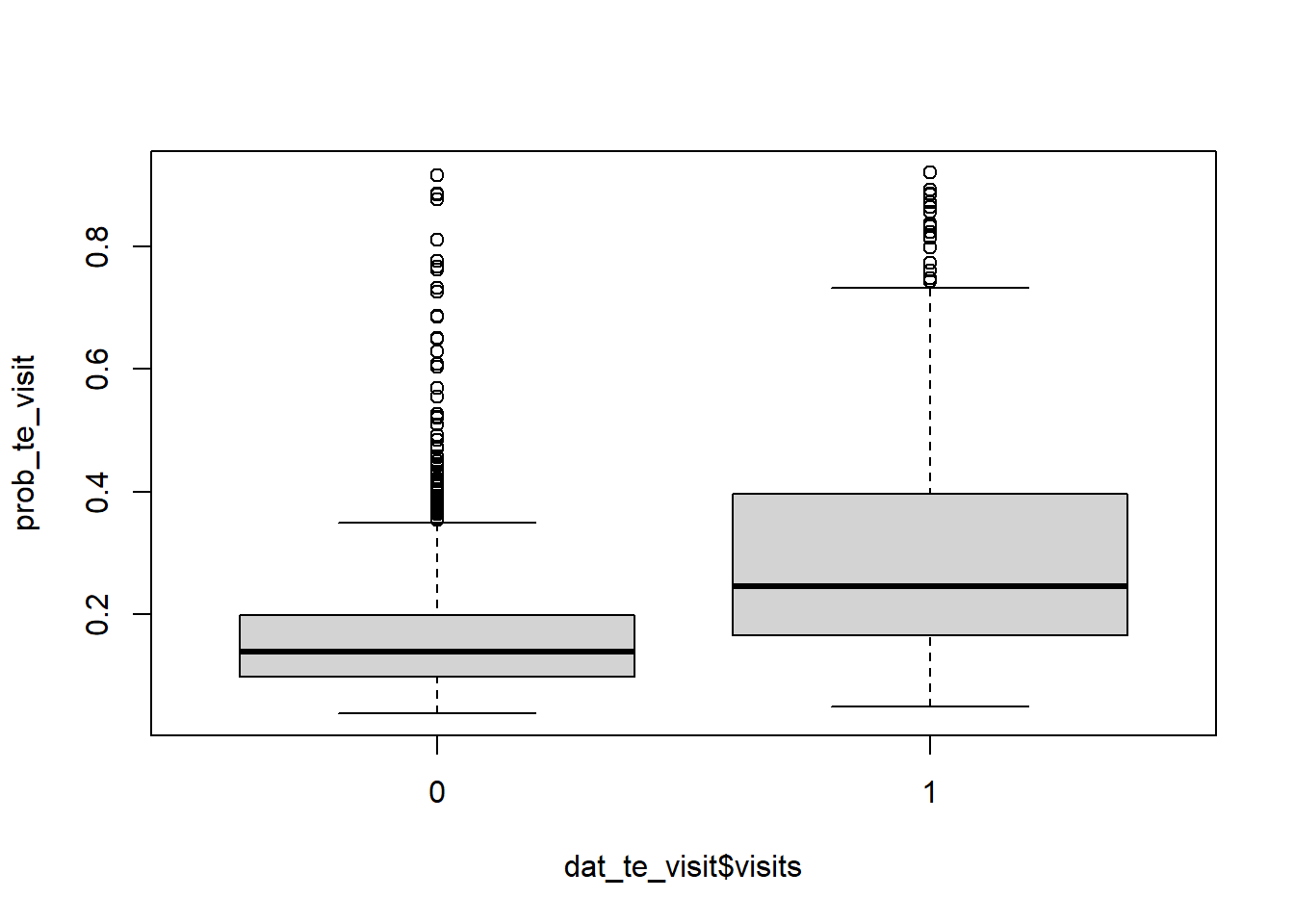
For now, this can be further inspected by looking at the predicted probabilities per observed label.
::: panel-tabset
### R
```{r}
boxplot(prob_te_visit~dat_te_visit$visits)
```
### Python
```{python}
#| label: visualize-prediction2
#| eval: false
fig, ax = plt.subplots()
ax.boxplot([prob_te_visit[r.dat_te_visit['visits']==0], prob_te_visit[r.dat_te_visit['visits']==1]]);
ax.set_xticklabels(['No Visit', 'Visit']);
ax.set_ylabel('Predicted Probability');
ax.set_title('Predicted Probabilities by Visit Status');
plt.show()
```
:::
We see that if the lowest predicted probabilities are usually assigned to 0-observations, most of the probabilities remain below 0.5 (even for the 1-observations). A good model would have two well separated boxplots, well away from 0.5.
Now, as an exercise, write down the prediction equation of the selected model, like you did for linear regression. Use this equation to explain how instance 1 and 2 (test set) are predicted, and calculate the predictions manually. Verify your results using the function *predict* used before.
<details>
<summary>Answer</summary>
```{r}
prob_te_visit[c(1,2)]
```
$$
z(x) = -2.31795-0.31838\times gender\_male+0.39762\times age+\\0.28431\times illness+0.16340\times reduced+0.05589\times health+\\0.27249\times private\_eyes -0.65344\times freepoor\_yes+\\0.38038\times freerepat\_yes
$$ Then $$
P(Y=1 | X=x) = \frac{e^{z(x)}}{1+e^{z(x)}}
$$
</details>
# LASSO & Ridge regressions
You have been introduced to lasso and ridge regression during the *Variable selection with penalization* part of the lecture.
Lasso and Ridge Regression are two regularization techniques used in regression models to prevent overfitting by adding a penalty term to the loss function. Lasso regression (aka $L_1$) adds a penalty term equal to the absolute value of the coefficients. In contrast, Ridge regression (aka $L_2$) adds a penalty term equal to the squared value of the coefficients. The effect of the penalty term is to shrink the coefficients towards zero, which can help reduce model complexity and improve generalization performance. In this case, we apply lasso and ridge to the real estate data and do not cover logistic regression (example already seen during the class).
First, we need to turn our predictors into matrices, as this is required by the `glmnet` package in R and works with the python implementation.
```{r}
# glmnet can only work with matrix objects, columns 2-7 correspond to the same ones used by `lm`
dat_tr_re_mat_x <- select(dat_tr_restate, c(2:7)) %>% as.matrix()
dat_tr_re_mat_y <- pull(dat_tr_restate,'Price')
dat_te_re_mat_x <- select(dat_te_restate, c(2:7)) %>% as.matrix()
dat_te_re_mat_y <- pull(dat_te_restate,'Price')
```
::: panel-tabset
## R
On the newly created matrices, we run cross-validated lasso and ridge with the `cv.glmnet()`, function where setting the `alpha` (penalty) parameter as 1 produces lasso regression and 0 produces ridge regression. The default value of alpha is 1, which corresponds to lasso regression. For 0<alpha<1, it performs Elastic Net regression (a combination of $L_1$ and $L_2$ regularization).
```{r}
# Load appropriate library and set a seed
library(glmnet)
set.seed(123)

# Fit Ridge regression model
ridge_fit <- cv.glmnet(x = dat_tr_re_mat_x, y = dat_tr_re_mat_y, alpha = 0)

# Fit Lasso regression model
lasso_fit <- cv.glmnet(x = dat_tr_re_mat_x, y = dat_tr_re_mat_y, alpha = 1) #if you change the `family` argument to `bionomial`, you can get also logistic regression
```
We can then fit the final models with the best parameters:
```{r}
ridge_fit_best <- glmnet(x=dat_tr_re_mat_x, y = dat_tr_re_mat_y,
                         lambda = ridge_fit$lambda.min)

lasso_fit_best <- glmnet(x=dat_tr_re_mat_x, y=dat_tr_re_mat_y,
                         lambda = lasso_fit$lambda.min) #can also use lasso_fit$lambda.1se
```
We can compare different performances for this task using `caret::postResample()`. We will learn more this function and it's metrics the upcoming courses & lab sessions.
```{r}
# lasso & ridge performance on the training set
caret::postResample(predict(ridge_fit_best, newx = dat_tr_re_mat_x), dat_tr_re_mat_y)
caret::postResample(predict(lasso_fit_best, newx = dat_tr_re_mat_x), dat_tr_re_mat_y)

# lasso & ridge performance on the test set
caret::postResample(predict(ridge_fit_best, newx = dat_te_re_mat_x), dat_te_re_mat_y)
caret::postResample(predict(lasso_fit_best, newx = dat_te_re_mat_x), dat_te_re_mat_y)

# Step-wise lm performance on training and test sets
caret::postResample(predict(mod_lm_sel,dat_tr_restate), dat_tr_re_mat_y)
caret::postResample(predict(mod_lm_sel,dat_te_restate), dat_te_re_mat_y)
```
In this case, the lasso is better than the ridge on the test set, and if you have many features, this could be a useful technique. However, they are both outperformed by step-wise linear regression. Lasso and ridge are more useful when you have many more variables. You can try this already by taking more variables for your `dat_tr_re_mat_x` and `dat_te_re_mat_x` such `select(dat_te_restate,-c('Price', 'Month'))` to see how (for better or worse) the performance changes. If you want more explanation on why linear model outperformed lasso and ridge, check out (click on) the further explanation below.
<details>
<summary>Why lm (or step lm) outperformed lasso & ridge </summary>
In some situations, it is normal to observe that a linear model may perform better than a regularized model, such as a ridge or lasso. This can occur when the number of predictors in the model is small relative to the sample size or when the predictors are highly correlated.
Linear regression assumes that the relationship between the response variable and the predictors is linear and additive. When this assumption holds, a linear model can be a good choice. In contrast, regularized regression methods such as ridge and lasso add a penalty term to the regression objective function to shrink the estimated coefficients towards zero, which can help to avoid overfitting when the number of predictors is large relative to the sample size or when the predictors are highly correlated.
However, when the number of predictors is small relative to the sample size or when the predictors are highly correlated, the additional regularization provided by ridge or lasso may not be necessary, and a simple linear model may perform better.
It is always a good practice to compare the performance of different models using appropriate evaluation metrics and techniques such as cross-validation. The choice of the best model will depend on the specific problem and the goals of the analysis.
</details>
## Python
```{python}
from sklearn.linear_model import Ridge, Lasso, RidgeCV, LassoCV
import numpy as np

# Set a seed for reproducibility
np.random.seed(123)

# Fit Lasso regression model
lasso_cv = LassoCV(cv=10)
lasso_cv.fit(r.dat_tr_re_mat_x, r.dat_tr_re_mat_y);

# Get the optimal regularization parameter
lasso_optimal_alpha = lasso_cv.alpha_

# Fit the Lasso model with the optimal alpha
lasso_best_py = Lasso(alpha=lasso_optimal_alpha)
lasso_best_py.fit(r.dat_tr_re_mat_x, r.dat_tr_re_mat_y);

# Fit Ridge regression model with cross-validation
ridge_cv = RidgeCV(cv=10)
ridge_cv.fit(r.dat_tr_re_mat_x, r.dat_tr_re_mat_y);

# Get the optimal regularization parameter
ridge_optimal_alpha = ridge_cv.alpha_

# Fit the Ridge model with the optimal alpha
ridge_best_py = Ridge(alpha=ridge_optimal_alpha)
ridge_best_py.fit(r.dat_tr_re_mat_x, r.dat_tr_re_mat_y);
```
The `lambda` argument in `cv.glmnet()` from R corresponds to the `alpha` argument in `RidgeCV()`/`LassoCV()` in python. In `cv.glmnet()`, the lambda argument specifies the range of regularization parameters to be tested in the model selection process. By default, lambda is set to NULL, which means that `glmnet()` will automatically choose a sequence of lambda values to search over. Note that in `glmnet()`, lambda values are used for both $L_1$ (lasso) and $L_2$ (ridge) regularization, whereas in `RidgeCV()`, alpha values are used to control the mix of L1 and L2 regularization, with alpha = 0 corresponding to pure L2 regularization (i.e., ridge regression).
On the contrary (and to avoid confusion), the `alpha` argument in `cv.glmnet()` corresponds to the `fit_intercept` argument in `RidgeCV()`/`LassoCV()`. In `cv.glmnet()`, the alpha argument specifies the mixing parameter between L1 and L2 regularization.
```{r}
# python lasso & ridge performance on the training set
caret::postResample(py$ridge_best_py$predict(dat_tr_re_mat_x), dat_tr_re_mat_y)
caret::postResample(py$lasso_best_py$predict(dat_tr_re_mat_x), dat_tr_re_mat_y)

# python lasso & ridge performance on the test set
caret::postResample(py$ridge_best_py$predict( dat_te_re_mat_x), dat_te_re_mat_y)
caret::postResample(py$lasso_best_py$predict(dat_te_re_mat_x), dat_te_re_mat_y)
```
The performance is different in python simply because of different default settings for the python vs R implementations.
:::
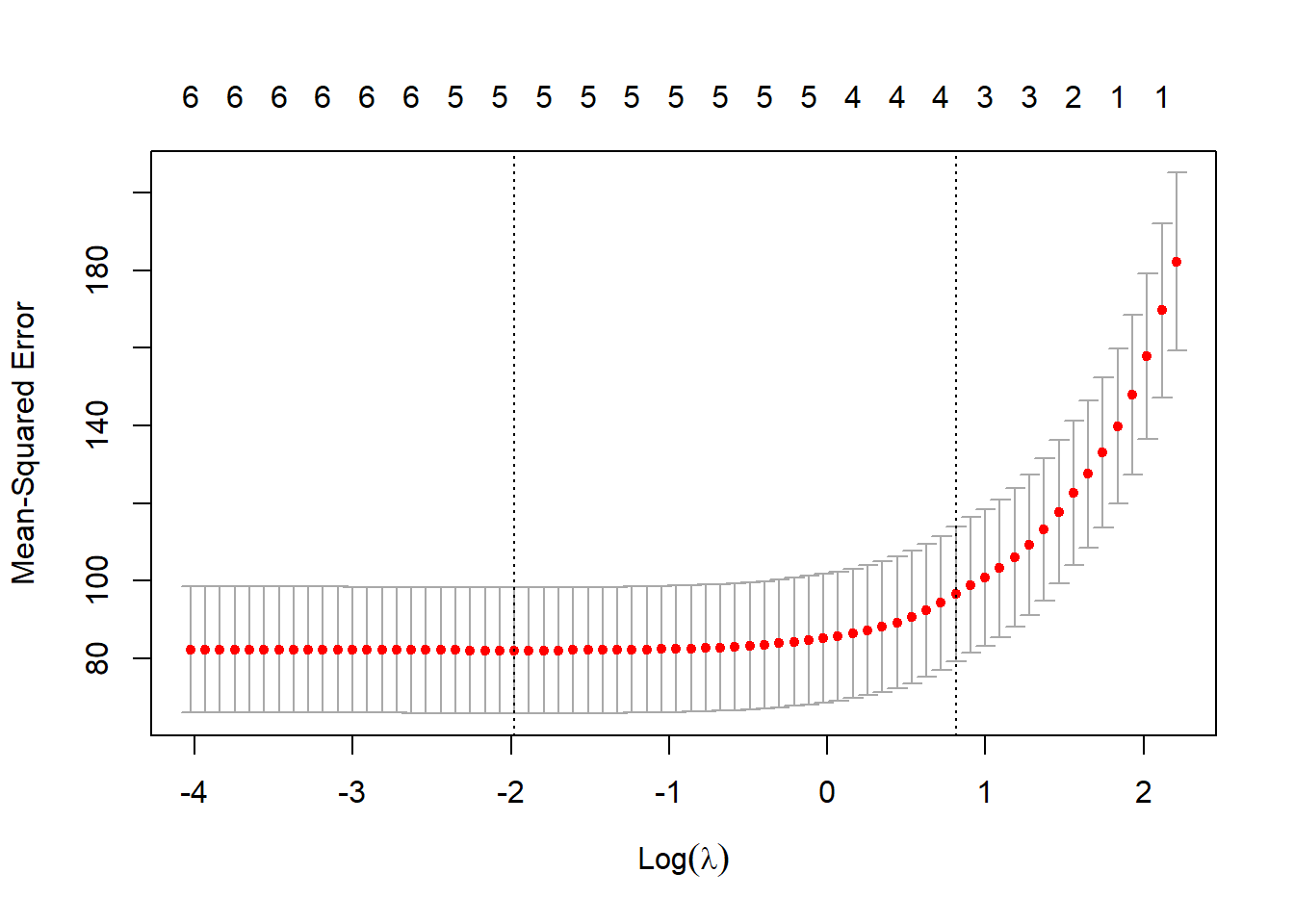
To understand the decision making of lasso, we can check the beta's in a similar fashion to a regression (only shown for the R models).
```{r}
# running the following can tell you a bit about the impact of different variables
small.lambda.index <- which(lasso_fit$lambda == lasso_fit$lambda.min)
lasso_fit$glmnet.fit$beta[, small.lambda.index]

# or on the final model
coef(lasso_fit , s= 'lambda.min')
plot(lasso_fit, xvar = "lambda", label = TRUE)
```
We can see that from the first output `Long` value has almost a beta of 0. In the second output, it is confirmed that the coefficient of this variable is indeed 0. This could explain why `mod_lm_sel` also dropped this variable. The rest of the coefficient are similar to `summary(mod_lm_sel)`. as ridge or lasso in some situations. This can occur when the number of predictors in the model is small relative to the sample size, or when the predictors are highly correlated.
# Your turn to practice
## Linear regression: nursing home data
Now it is your turn. Make an linear regression (also feel free to try lasso and ridge regressions) on the nursing data described below (found also in `/data/nursing_data.csv`). Afterwards, use linear regression to build a predictor of the cost using the other features. Replicate the analysis. Split the data, build a model, make the variable selection, make the predictions and analyze the results. Make also an analysis of the coefficients in terms of the associations between the costs and the features.
<details>
<summary>Data Description</summary>
The data set is about patients in a nursing home, where elderly people are helped with daily living needs, also known as Activities of Daily Living (ADL, i.e. communication, eating, walking, showering, going to a toilet, etc.).
Since the stay in such facilities is very expensive, it is important to classify the new-coming patient, and estimate the duration of the stay and the corresponding costs.
In practice, there are different types of patients who require different types of help and, consequently, different duration of the stay. For example, there could be a person with severe mobility issues, who requires the help with most of the needs every day; or a person with mental deviations, who don't need help with daily routine, but requires extra communication hours.
Here, we will focus of total amount of help (measured in minutes of help provided to a person per week) provided and measure the costs of stay of a person.
The data set on which the analysis is based has the following columns:
- **gender**: a categorical variable with levels "*M*" for male and "*F*" for female
- **age**: integer variable
- **mobil**: categorical variable that represents the physical mobility with levels
- 1 = Full mobility
- 2 = Reduced mobility
- 3 = Restricted mobility in the house
- 4 = Null mobility
- **orient**: categorical variable that represents the orientation (interactions with the environment) with levels
- 1 = Full orientation
- 2 = Moderate disturbance of orientation
- 3 = Disorientation
- **independ**: categorical variable that represents the independence of ADL with levels
- 1 = Independent of help
- 2 = Dependent less than 24 hours per day
- 3 = Dependent at unpredictable time intervals for most of the needs
- **minut_mob**: numerical variable that represents the total number of minutes of help with movement per week
- **need_comm**: categorical variable with levels "*Yes*" for a person who needs extra communication sessions with an employee, and "*No*" otherwise
- **minut_comm**: numerical variable that represents the total number of minutes of communication per week
- **tot_minut**: numerical variable that represents the total number of minutes spent on a patient per week, $tot\_minut = minut\_mob + minut\_comm$
- **cost**: numerical variable that represents the total costs of having a patient in the nursing house per month.
</details>
Note: since tot_minut=minut_mob+minut_comm, you may not find any meaningful result using the 3 features. This is perfectly normal. Just use 2 features only among these 3 (arbitrary choice).
## Logistic regression: the credit quality
The German Credit Quality Dataset consists of a set of attributes as good or bad credit risks. In order to find find a detailed description of the features, please refer to the [original link to the dataset](https://archive.ics.uci.edu/ml/datasets/statlog+(german+credit+data)). The `german.csv` file can also be found in `/data/german.csv` whichis the mdified version of the original dataset to simplify the analysis, especially the data loading in **R**.
The aim here is to predict the credit quality from the other features. The outcome **Quality** is 0 for "bad" and 1 for "good". Make an analysis of the data and develop the learner. You can follow these notable steps:
- Make a simple EDA of the features
- Split the data and train the model.
- Make variable selection and check out the result.
- Interpret the coefficients.
- Inspect the quality of the model by making the predictions (confusion table and boxplot of the predicted probabilities).
Note that the data are unbalanced again and that you may not find a very good predictor. This issue is quite difficult and will be addressed later.
